I find political / ideological surveys nearly impossible to complete, because every possible answer mischaracterises me in some way. Some questions are about policy and others about values, and the purpose of the whole thing is to assign you to an appropriate political “tribe”, but my values and policy preferences turn out to be inconsistent and very dependent on how I interpret the question. Whether my interpretation matches that of others is down to luck, so I usually give up in frustration about halfway through.

As a reflection of this, on my Twitter profile I say I’m “liberal conservative”, which doesn’t mean anything to anyone. Let me try to explain.

On most policy-level questions I side with liberals. Drug decriminalisation? Yes please. Make markets as free as possible and use them as much as possible? Sure. Allow a market in human organs for transplantation? Yes, it would make everyone better off. No to trade barriers and protectionism? Absolutely. Decriminalize victimless crimes? Yes, except if that turns out to have really bad consequences. Privatize everything? Yes, up to a point, ownership promotes preservation and efficient use. State-owned resources are usually wasted horrendously and become political pawns.

These positions could be summed up as liberalism, perhaps “right liberalism” or “neoliberalism”. Add to this a resource redistribution scheme that prevents poverty (because poverty leads to disharmony and conflict, which is the ultimate evil), and schooling and public amenities enough to allow for social mobility (because desperation leads to disharmony and conflict), and you have roughly what people in the 1990’s thought the 2010’s was going to look like. Didn’t turn out that way, of course..
But I’m not liberal, I’m conservative! How can that be?

The reason I favour non-interventionism in general is that I have low confidence in the ability of human planners to discover and enforce good rules. And enforcing always involves the implicit use of violence, which to me seems prima facie extreme and unconservative.

I am more inclined to trust in organically evolved institutions and customs, both in that they are a better fit to human nature and in that they take into account local variations better than statewide rules can. An illustrative quote from Alexander Hamilton:

If men were angels, no government would be necessary. If angels were to govern men, neither external nor internal controls on government would be necessary. In framing a government which is to be administered by men over men, the great difficulty lies in this: you must first enable the government to control the governed; and in the next place oblige it to control itself.

I’m also conservative in the deep-down sense that my beliefs about a good life and a good society are conservative. I value caution, preservation, moderation and modesty. I think people should be very cautious about drugs, drink and gambling, and that it is a moral failing to allow your life to be destroyed by them; that polyamory is usually a façade for charismatic people to have sex with a lot of people who tolerate their situation but are harmed by it in the long term; that easy living and decadence in immoderation are harmful both to individuals and societies; that responsibilities come before happiness; I’m upset about divorce and adultery; I believe that everyone is responsible not just to the present moment but to the past and to the future. And so on and so on. My hope is that non-interventionism on the part of the state would lead to some more conservative outcomes, at least for those who would benefit from them. Many of the things I mentioned are either made worse or not helped by government intervention. I don’t want to impose these things on everyone, but I think communities with such values have a place in the world.

These positions could be called not just conservative, but moralistic. I am gung-ho about participating in social control to make people stay in line regarding these things, especially given that I am unwilling to use government force to do so. My positions even become nationalistic when you add in responsibilities from the past, like the responsibility to preserve one’s culture, nation, independence etc. And to the future also belongs the natural world, to which we don’t have the right to do anything we will. Another illustrative quote, from Jonathan Haidt, who is not conservative but a liberal / moderate social scientist trying here to sum up what conservatives believe:

Conservatives believe that people are inherently imperfect and are prone to act badly when all constraints and accountability are removed. Our reasoning is flawed and prone to overconfidence, so it’s dangerous to construct theories based on pure reason, unconstrained by intuition and historical experience. Institutions emerge gradually as social facts, which we then respect and even sacralize, but if we strip these institutions of authority and treat them as arbitrary contrivances that exist only for our benefit, we render them less effective. We then expose ourselves to increased anomie and social disorder.

And here’s Oakeshott:

To be conservative is to prefer the familiar to the unknown, to prefer the tried to the untried, fact to mystery, the actual to the impossible, the limited to the unbounded, the near to the distant, the sufficient to the superabundant, the convenient to the perfect, the present laughter to the utopian bliss.

So I’m really conservative in terms of values, but thinking about things tends to lead me to liberal positions. You could say I’m liberal because I’m conservative!

Another interesting case is moral philosophy. I mostly judge people on whether they do (what I consider to be) their duty towards others, and whether they are virtuous in their actions. These moral positions are deontological ethics and virtue ethics, respectively. The other major position is consequentialism (or utilitarianism), that actions should be judged on their consequences. The greatest good for the greatest number. Doesn’t that sound logical? What is virtue, duty or a rule-book when children starve and preventable diseases kill? Why am I not a consequentialist?

Ultimately it’s because I don’t believe people are very good at doing difficult moral calculations, and that even if they were good at it, they wouldn’t want to behave according to the calculations anyway. It’s a limitation of human nature. On the other hand, people are good at aspiring to celebrated virtues & policing each other about their obligations, trying make make themselves look good and ostracising those who don’t. In other words, deontological ethics and virtue ethics actually work.

So… if I believe in virtue ethics and deontological ethics because it ultimately leads to the greater good, does that make me a consequentialist in the end? Maybe. Sort of. It sure makes it hard to directly answer questions about it.

There’s a pattern here that I find interesting. There’s the private / internal / fundamental level, which after interacting with facts about the outside world and logic is transformed, possibly into something like its opposite. Often I think disagreements about values are really about people meeting each other on the wrong level of thinking, or people disagreeing about facts (like the implications of human nature). Here’s one more example.

Am I a feminist? Well, no. At least in the sense that when something is described as a “feminist goal”, like having lots of women on the boards of corporations, or having female movie stars earn the same as male movie stars, I generally roll my eyes and hope the whole thing just goes away. Or in the sense of equality. I hardly know what it means as a policy position – that the sexes are different from each other is to me as clear as day, so it would seem that they can hardly be equal in any meaningful sense.
Then again, it’s easy to agree with definitions of feminism along the lines of “when gender is not essentially important, people should not be discriminated on the basis of gender”. I am not the sort of antifeminist who wants a male head of state or who would resent a female boss, and I think hardly anyone is these days. I live in a feminist society and have to some extent internalised its values, and I’m in no way the head of my own household (it’s just not up to me).

I suspect that in the absence of discrimination we would continue to see men be a disproportionate part of the top echelons of society (and of every profession, sport and hobby) – and also of the bottom, where they make up almost all of the prisoner and homeless population. But if it turned out that everything becomes perfectly statistically equal, I’d be ok with that.

So if you want to turn me into a feminist (in the sense of agreeing with public intellectuals about feminism-related topics), it’s not sufficient to change my values – you’d have to change my facts (that men and women are different) or my thinking.

I have been listening to a lot of (many versions of) Eyes Of The World (a Grateful Dead song, natch). A really intense and fast one from 1978 (Red Rocks Amphitheatre July 7th) and a really slow jazzy one by Dead & Co. from last summer in particular – but all kinds.

The words, written by Robert Hunter — who was not in the band, but was a frequent lyrical collaborator — are supposed to have some sort of Buddhist awakening message, but I think I’ve gotten into them from a parenting perspective. Children being the ultimate experiencers, fresh with promise, so innocent of everything — including their own feelings which, at once deeply authentic and coming and going like the weather, they express in unsure imitations of other people — that they don’t really understand either their internal world or the outside world. Desperately needing guidance, but barely capable of receiving it, in the end you’re left exhausted and wondering what your standing to guide anyone is anyway.

“Eyes” evokes in me the kind of fundamental (and I mean fundamental, as in “what are feelings, what are thoughts, what is life”) guidance I’d like to give, but they’re three and zero years old, and I don’t know is it possible to guide anyone in that anyway. So let me just write down my thoughts, in [bracketed italics] about the lyrics before I forget them. If you want to follow along, that ‘78 Eyes is here (just click on it in the playlist). Go loud!

[First, there’s a beautiful bit of scene-setting.]

Right outside this lazy summer home
  you don’t have time to call your soul a critic, no
Right outside the lazy gate of winter’s summer home
  wondering where the nuthatch winters
  wings a mile long just carried the bird away

[The first line makes me think it’s my home we’re outside, in the garden, in summer, on holiday. An uncritical, open setting. Why, then don’t I have *time* to call my soul a critic – and does that imply that my soul *is* a critic? I think so. The soul is critical, but I don’t silence it or challenge it. That would lead to nothing, and be a waste of time.

Then, “Right outside the lazy gate of winter’s summer home”. What’s a lazy gate? In summer, winter is surely on holiday. Or in the southern hemisphere? Winter is that which drives birds to migrate. Some things exclude each other, but they can still wonder about one another.]

Wake up to find out that you are the eyes of the world
  but the heart has its beaches its homeland and thoughts of its own
Wake now, discover that you are the song that the morning brings
  but the heart has its seasons, its evenings and songs of its own

[Wake up = become more conscious, notice your feelings, focus your mind. You will find out that in your life, you are the unique locus of experience but also part of the world. Your world “sees itself” through you, and in experiencing the world, you make it exist.

But the heart has its seasons, its evenings and songs of its own = but you’re not in control, your self-creation and unpredictable change will continue indefinitely.]

There comes a redeemer
  and he slowly too fades away
There follows a wagon behind him
  that’s loaded with clay
And the seeds that were silent
  all burst into bloom and decay
The night comes so quiet
  and it’s close on the heels of the day

[There comes a redeemer and he slowly too fades away – I think this is something like inspiration, insight, excitement. Or some sort of big idea you commit yourself to. It comes, and it’s important, but it doesn’t last forever. The wagon loaded with clay could be the mundane. The whole thing is like an inversion of creation: the world is made of clay, and is preceded by a redeemer.
The seeds that were silent = While you were excited by the big thing, smaller things were waiting inside. Perhaps they were planted in the mundane clay. They burst into bloom and decay (everything ends, and the cycle starts again).
The night comes so quiet = endings come unannounced and you might only notice them when they’ve already happened.]

Wake up to find out that you are the eyes of the world
  but the heart has its beaches its homeland and thoughts of its own
Wake now, discover that you are the song that the morning brings
  but the heart has its seasons, its evenings and songs of its own

Sometimes we live no particular way but our own
Sometimes we visit your country and live in your home
Sometimes we ride on your horses
Sometimes we walk alone
Sometimes the songs that we hear are just songs of our own

[In some situations you’re an individual
In others you’re groupish or depend on other people
When you get to benefit from the world around you, that’s powerful
Sometimes you’ll go the other way and it’s harder
It’s hard to tell what’s coming to you from the outside vs. the inside

(I should have been a poet..)]

Wake up to find out that you are the eyes of the world
  but the heart has its beaches its homeland and thoughts of its own
Wake now, discover that you are the song that the morning brings
  but the heart has its seasons, its evenings and songs of its own

And of course, just because I can’t explain this to my children doesn’t mean we can’t party!

I’ve just finished Geoff Hinton’s neural networks course on Coursera. It’s been considerably tougher than the other courses I’ve done there; Andrew Ng’s machine learning course and Dan Jurafsky & Chris Manning’s natural language processing course.

Whereas the other courses could serve as theory-light introduction for people who only have experience as coders, Hinton’s course expects basic understanding of probability and linear algebra and the ability to calculate non-trivial partial derivatives. There was a lot of supplementary material, including research papers and optional extra projects. I think I spent just a few hours on them, but I could have easily spent 20-30.

All of the above-mentioned people are leading researchers in their fields, and it’s pretty amazing that this material is available free of charge. This is something you just couldn’t get at eg. the University of Helsinki where I work. If you’re not familiar with Coursera, there are video lectures with mini-quizzes, reading material, more involved weekly exams, programming assignments and final quizzes, all nicely integrated.

You have to get at least a 80% score on each exam and assignment to pass, which is close to “mastery learning”, which I think is a good idea. This is in contrast to regular schools, where you might get a 50% score and then just keep moving on to more difficult material. To get mastery learning right, you have to allow exam retakes, which requires a large number of possible exams so that students can’t get a perfect score by just trial and error. This course didn’t completely achieve that, leaving it partly down to the student not to resort to trial and error.

By the way, don’t confuse mastery learning, which has to do with humans studying, with machine learning or deep learning, which are computational techniques to get computers to do things!

I’ve also attended a study group on the “Deep Learning Book” (henceforth DLB), and followed Andrej Karpathy’s lectures on convolutional neural networks (henceforth CNN) (which I think are no longer freely available because they didn’t have subtitles and so deaf people couldn’t watch them, so Stanford had to take them down – but I have copies). I’m going to do a little compare & contrast on these neural networks study resources. There is a lot of jargon, but at the end I’ll include an “everyman’s glossary” where I try to explain some concepts in case you’re interested in this stuff but don’t know what the things I’m talking about mean.

***

Hinton’s career has mostly been in the era of neural networks showing great promise but not quite working, and he tells you a lot about what hasn’t worked historically. Even things like backpropagation, which is used everywhere now, was developed and abandoned in the 80’s when people decided that it was never going to work properly. Other resources just tell you what works great, but leave out a lot of details about how careful you have to be to get things started the right way.

DLB is rather focused on feedforward nets and variations of them, all trained with backpropagation, and of course CNNs are the main feedforward model for anything having to do with visual data. Even recursive networks are presented as an extension of feedforward nets, which is not the way things developed historically.

Hinton presents a much more diverse cast of models, some of which were completely new to me, eg. echo state networks and sigmoid belief nets. Some of the time I was thinking “If this isn’t state-of-the-art, am I wasting my time?”, but ultimately all the material was interesting.

DLB and Karpathy made everything seem intuitive and “easy”, presenting a succession of models and architectures getting better and better results. Hinton made things seem more difficult and made you think about the mathematical details and properties of things much more. If you like engineering and results, go for DLB and the CNN course (and the Ng machine learning course first of all) – if you like maths, history and head-scratching, go for Hinton.

Hinton uses restricted Boltzmann machines (henceforth RBM) a lot. They are introduced via Hopfield nets and general Boltzmann machines, and used especially for unsupervised learning and pre-training. They are trained with something called contrastive divergence, an approximation technique that was new to me. Weight sharing is a recurring theme, used to develop intractable “ideal” models into practical models with similar characteristics. Dropout, which in DLB is just a normalization technique, is derived by Hinton as combining an exponential (in number of units and dropout) number of models with weight-sharing. ReLu units, which are introduced in DLB in an extremely hand-wavy way, are actually derived by Hinton as a limiting case of using multiple logistic units in parallel.

DLB and Karpathy mostly ignore the topic of weight initialization, saying that it’s no longer necessary. With Hinton it’s more central, probably because that was how the deep neural network revolution got really going originally. He points to architectures that were promising but didn’t work in the 80’s – 90’s but started working better with eg. RBM pretraining + backprop fine-tuning. Later he says that a stack of denoising or contractive autoencoders probably works even better for pretraining.

I found the pretraining methods interesting from a cognitive science standpoint. Denoising autoencoders lead to models where all the neurons are forced to model correlations between features, and RBMs & contractive autoencoders tend to lead to “small active sets”, where most of the hidden layer is insensitive to most inputs.

Hinton’s “final conclusion” about pretraining is that it will continue to be useful for situations where you have a smaller amount of labeled data and a larger amount of unlabeled data. With unsupervised pretraining you can still use the unlabeled data, which surely contains valuable information about the data space. That’s probably true, but I guess with images we now have enough labeled data.

The other problem for which pre-training is useful is very deep nets where the learning gradients vanish if you initialize all weights to be small random weights. I understand that this is now handled by directly connecting far-apart layers to each other, allowing information about the data flow both through deeper and shorter stacks of neurons.

Hinton reports that he’s had arguments with people from Google saying that they no longer need pretraining OR regularisation because they have such a huge amount of labeled data that they won’t overfit. Hinton argues that once they use even bigger and deeper networks they’ll start overfitting again, and will need regularisation and pretraining again, and I think that has happened (Hinton’s course is from 2013), at least for regularisation.

Hinton has some quite demanding programming exercises with little guidance, sometimes too little. Different regularisation methods are covered, including somewhat obsolete ones like early stopping, and you get a good overview of the differences. The exams are a mixed bag – many annoying underspecified questions with gotcha-answers, but also good mathy ones where you have to get a pencil and paper out.

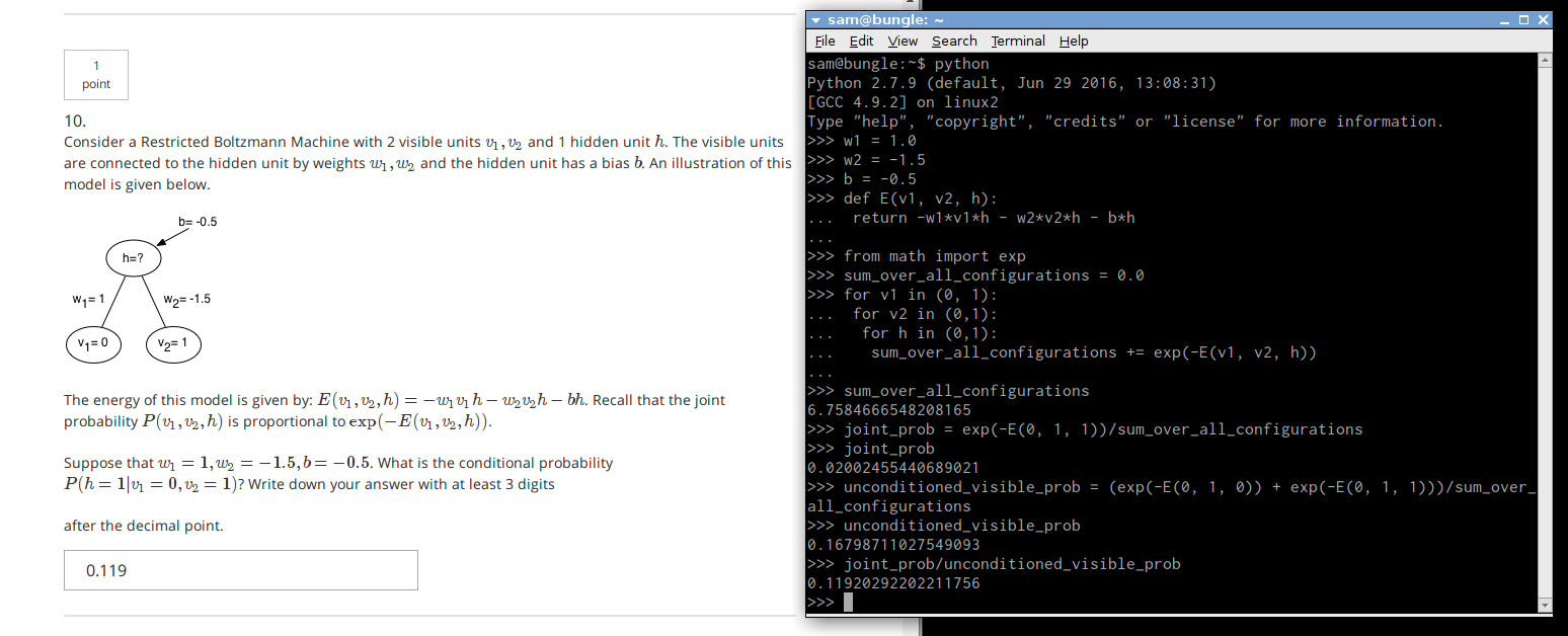
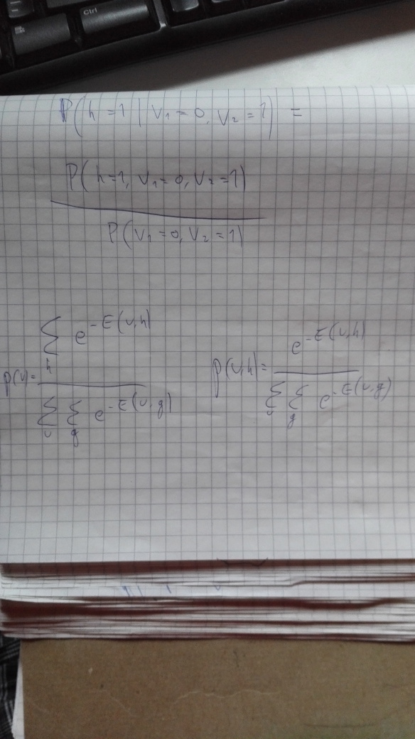
Here’s an example – it’s not really hard, but you have to think back quite far in the course and do some actual calculations. The screenshot shows the problem and the way I calculated the solution. The scribbles on the notepad show formulating the conditional probability that the question is about in terms of the probability of the joint configuration and the probability of just the visible units, and showing the probabilities of those in terms of the energy function E. Click to enlarge.

Whereas Hinton has quite a lot of emphasis on doing math by hand, rather than eg. just using software to handle everything via backprop, DLB is more oriented towards the engineering and applications side. Hinton has you not just calculating gradients, but deriving and proving properties of what learning does to the network etc.

Hinton does cover CNNs as well, but in a more theoretical way, not covering a litany of models and approaches. He shows AlexNet from 2012, and then later when covering image retrieval he first training a deep autoencoder to hash images into binary codes and uses Hamming distance to find matches. This works, but is a lot less impressive than the state of the art. Then he swaps out the image data his autoencoder is getting for the activations from AlexNet and gets a really good image retrieval system. A nice example of the development of the field.

***

An everyman’s glossary

Neural network: a system that connects individual units of very simple computation together in order to get the network of these units to accomplish some more complicated task. These systems are behind things like Google image search, self-driving cars and recommender systems that try to predict what you’re interested in buying next.

Objective function / loss function: a way to measure what you’re trying to achieve. Eg. if you’re trying to detect objects in pictures, the objective function measures how well your system did at detecting objects in pictures where the content is already known. This is called “supervised learning”.

Backpropagation: a way to determine for each part of the network what way it should change in order to better satisfy the objective function. This involves calculating the derivative of the objective function with respect to the parts immediately before the output layer, and then re-using those derivatives to calculate the derivatives for parts further along in the network. If you remember the “chain rule” from calculus in school, this is essentially doing that over and over again.

Feedforward net: a neural network architecture where the input data is one layer and influences neurons on the next layer, which influences the next layer etc. Each connection between neurons is a “weight”, which is a number used to multiply the activation from the output-neuron and fed into the input-neuron. The final layer is the “output layer”. No backwards connections. A model like this is usually learned by using backpropagation to compute gradients (how should we change the weight) from the objective function to each weight, and then optimizing the weights using that.

Deep net: this just means that there are multiple layers of “hidden neurons”, meaning units that aren’t part of the input or the output of the system. Training (ie. finding good weights) a net like this is “deep learning”.

Optimization: in the context of neural networks, a method for finding good weights for all the connections in the network, given the gradients of the objective function with respect to each connection. Some version of “gradient descent” is typical. This is changing all the weights a small step in the direction of their respective gradients, recalculating the gradients, taking another step etc. until the objective function doesn’t get any better anymore.

Activation function: this is what a neuron does to its inputs to determine its own activation. For example, linear activation is taking each input, multiplying it by a weight and adding all of those together. This is linear because it can just scale the previous activations to be bigger or smaller. Its graph is a straight line. Complicated problems require nonlinear activations, like the logistic function, which has an S-shaped graph.

Unsupervised learning: this is where you don’t have an objective function, but are just trying to understand the data in some way. This can be useful for pretraining deep supervised networks.

Pretraining: in deep nets, it is sometimes difficult to get training to work because the hidden layers can be many layers separated from the output layer, where the objective function is calculated. In pretraining you first train the hidden layers separately to model the previous layer well (in an unsupervised way, without caring about the objective function), and then finally you stack them together and use backpropagation to fine-tune the system with the objective function.

ReLu / rectified linear unit: the simplest kind of nonlinear activation function. When the input is negative, it outputs zero, and when the input is positive, it outputs the input. The graph is two straight lines put together, with one point of nonlinearity (and noncontinuity). Very commonly used today.

RBM / Restricted Boltzmann Machine: an undirected neural network, where connections between neurons are two-way (but with just one weight covering both directions), and the whole system is made to minimize an “energy function”, making the configurations of the whole system conditional on the given data simple and probable. The “restricted” part means that there are no connections between hidden units, just between the inputs and the hidden units.

Underfitting / overfitting: underfitting is when the system is unable to model structure in the data because it doesn’t have enough modeling capacity. Overfitting is when the system has so much capacity it models even random correlations in the data, leading to bad performance when new data doesn’t have those random correlations. This is remedied by using regularisation techniques, like adding terms to the objective function making the network want to be simpler and more generalising.

Autoencoder: a system that uses an input to reproduce itself via some simpler intermediate representation. For example, taking 256-by-256 pixel images, encoding them into a vector of 20 numbers, and trying to use that encoding to reproduce the original image as well as possible.

Tell me if I’m missing something important from the glossary.